Vector search (ANN)
What is vector search?
Vector search finds the items whose vectors sit closest to a query vector. You turn a piece of text, an image, or a question into a vector with an embedding model, then ask the search to return the nearest vectors to it. Because vectors that mean similar things sit near each other, the nearest neighbours are the most relevant results, even when they share no words with the query.
Every candidate vector is scored against the query vector with a distance or similarity measure, and the closest handful come back. Search "waterproof cycling jacket" and a product listed as a "rain poncho for bikes" can rank first, because the model placed the two descriptions close together.
Vector search is the algorithm, not the storage. A vector database is the system that holds the vectors and runs the index; vector search is the retrieval step that runs on top of it. It is the same step that retrieval-augmented generation (RAG) uses to pull the passages a language model needs to ground its answer.
Why exact search does not scale
The exact answer is easy to define. Compare the query vector against every stored vector, sort by distance, and keep the closest k. This is exact k-nearest-neighbour search, or exact kNN, and it always returns the true nearest neighbours. FAISS calls this a flat index, and PostgreSQL's pgvector gives it to you whenever you query without an index: perfect recall, every time.
The problem is cost. Exact kNN touches every vector, so the work grows linearly with the size of the collection. With ten million vectors, one query computes ten million distances; double the collection and the query takes twice as long. At a few million items that is already too slow for a chat box or a busy catalogue that has to answer in milliseconds.
Production systems solve this with approximate nearest neighbour search, or ANN. An ANN method skips most of the comparisons and still returns almost the same neighbours, in a fraction of the time. You trade a small amount of accuracy for a large speed gain, and the amount you trade is tunable: let the search look wider and it approaches the exact answer, keep it narrow and it stays fast. The accuracy you keep is measured as recall against exact kNN, so exact search stays useful as the yardstick you check the approximation against.
The main index families
An ANN method needs an index: a structure built ahead of time that lets a query avoid scanning everything. Three families cover most of what you will meet.
HNSW (Hierarchical Navigable Small World) builds a layered graph where each vector links to its near neighbours. A query starts in a sparse top layer, takes a few long hops across the space, then drops through the layers until it settles on the closest points. The structure was introduced by Malkov and Yashunin, who showed the search cost grows roughly with the logarithm of the collection rather than linearly. The honest trade: the whole graph has to sit in memory for the fast random access to work, so HNSW buys its high recall and low latency with RAM.
IVF (inverted file) splits the vectors into cells, each grouped around a centroid found by clustering. A query first picks the few cells nearest the query vector and compares only against the vectors inside them. The catch: it is lighter on memory and quicker to build than a graph, but a neighbour that falls just across a cell boundary is missed unless you tell the query to probe more cells, which costs speed.
Quantisation pulls a different lever. Instead of changing how you search, it shrinks each vector, storing the numbers with fewer bits so far more of them fit in memory. The cost: distances are now computed on rounded vectors, so recall drops, which is why quantisation usually rides on top of an IVF or HNSW index rather than being used on its own.
Choosing a similarity metric
Nearness has to be defined by a metric, and three of them show up almost everywhere.
Cosine similarity measures the angle between two vectors and ignores their length. A long document and a short note on the same topic point the same way, so cosine treats them as close.
Dot product (inner product) folds in length as well as angle. For vectors already normalised to length one it gives the same ranking as cosine, a little faster.
Euclidean distance (L2) measures the straight-line gap between the two points, and it is the default in many libraries.
The metric is not a free choice: it has to match the one the embedding model was trained for. Azure OpenAI's embedding models, for example, are built for cosine, so scoring them with Euclidean distance ranks results worse for no reason. Check the model card before you configure the index, because switching the metric later means rebuilding it.
Hybrid search combines keyword and vector
Pure vector search has a blind spot: exact strings. A part number like BRK-4471, an acronym, or a rare surname does not always land near its matches in vector space, because the embedding model was trained on meaning rather than exact spelling. A classic keyword index handles those cases well.
Hybrid search runs both at once, a keyword index such as BM25 alongside vector search, and merges the two result lists, often with reciprocal rank fusion. In practice this beats either method on its own: Azure AI Search reports that hybrid queries with semantic ranking gave the most relevant results in its own benchmarks. A reranking step can then reorder the merged list before it is handed on.
Keywords
vector search
ann
approximate nearest neighbor
hnsw
ivf
embeddings
vector database
rag
hybrid search
reranking
semantic search
ai
From the blog.
More pieces from the field on the same topic.
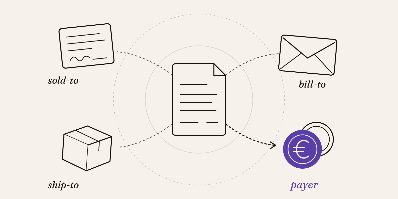
Sold-to, ship-to, bill-to and payer in SAP: who is actually your customer?
Sold-to, ship-to, bill-to and payer in SAP explained with a concrete example: who gets the invoice, whose account the receivable sits on, an...
New Data Panda connectors in August 2026
Seven new Data Panda connectors from August 2026: ECB rates, ProfitPlus Webshop, SAP S/4HANA, Exact Venice, OpusFlow, ABAX and Sprout Social...